The Bias-Variance Decomposition Demystified

Introduction

The generalisation error of a machine learning algorithm measures how accurately the learning algorithm is able to predict the outcome of new data, unseen during training. The bias-variance decomposition shows the generalisation error as the sum of three terms: bias, variance, and the irreducible error.

$$\tag{1} \text{Generalisation error} = \text{Bias}^2 + \text{Variance} + \text{Irreducible Error}$$

In many statistics and machine learning texts, this decomposition is just presented and its derivation skipped. In texts where it derived, it is often presented in a way that is inaccessible to many people. And why is it important to understand this derivation? Because the decomposition is a useful theoretical tool for understanding the performance of a learning algorithm. Understanding how bias and variance contribute to generalisation error helps us understand underfitting and overfitting.

The goal of this article is to present the bias-variance decomposition in an accessible and easy-to-follow format. We will restrict our discussion of this decomposition to regression problems where mean squared error is used as the performance metric.

A Quick Statistics Refresher

We will go over some statistics concepts that will aid our understanding of the other concepts we will discuss.

Expectation of a random variable

The expectation¹ or expected value of a random variable $X$, written as $\mathbb{E}[X]$, is the mean of a large number of observations of the random variable. The expectation has some basic properties:

• The expectation of any constant $c$ is the constant:

$$\tag{2} \begin{aligned} \mathbb{E}[c] = c \end{aligned}$$

$\mathbb{E}\big[\mathbb{E}[X]\big] = \mathbb{E}[X]$ because the expection of a random variable is a constant.

• Linearity of expectations: For any random variables $X$ and $Y$, the expectation of their sum is equal to the sum of their expectations:

$$\tag{3} \begin{aligned} \mathbb{E}[X+Y] = \mathbb{E}[X] + \mathbb{E}[Y] \end{aligned}$$

• For any random variable $X$ and a constant $c$:

$$\tag{4} \begin{aligned} \mathbb{E}[cX] = \mathbb{E}[c]\mathbb{E}[X] = c\mathbb{E}[X] \end{aligned}$$

Variance of a random variable

The variance of a random variable $X$ is the expectation of the squared difference of the random variable from its expectation $\color{blue} \mathbb{E}[X]$. In other words, it measures on average how spread out observations of the random variable are from the expectation of the random variable.

$$\begin{aligned} \tag{5} \text{Var}(X) & = \mathbb{E}\Big[\Big(X - {\color{blue} \mathbb{E}[X]}\Big)^2\Big] \\ & = \mathbb{E}\Big[\Big(X - {\color{blue}\mathbb{E}[X]} \Big)\Big(X - {\color{blue} \mathbb{E}[X]}\Big)\Big] \\ & = \mathbb{E}\Big[\Big(X^2 - 2X{\color{blue}\mathbb{E}[X]} + {\color{blue}\mathbb{E}[X]}^2\Big)\Big] \end{aligned}$$

If we recall that the expectation of a random variable $\color{blue}\mathbb{E}[X]$ is a constant and if we use the properties stated in equations (3) and (4), we get:

$$\tag{6} \begin{aligned} \text{Var}(X) & = \mathbb{E}\big[X^2\big] - \mathbb{E}\big[2X{\color{blue}\mathbb{E}[X]}\big] + \mathbb{E}\big[{\color{blue}\mathbb{E}[X]}^2\big] \\ & = \mathbb{E}[X^2] - 2{\color{blue}\mathbb{E}[X]\mathbb{E}[X]} + {\color{blue}\mathbb{E}[X]}^2 \\ & = \mathbb{E}[X^2] - 2{\color{blue}\mathbb{E}[X]}^2 + {\color{blue}\mathbb{E}[X]}^2 \\ \text{Var}(X) & = \mathbb{E}[X^2] - {\color{blue}\mathbb{E}[X]}^2 \end{aligned}$$

We could rewrite equation (6) as:

$$\tag{7} \begin{aligned} \mathbb{E}[X^2] & = \text{Var}(X) + {\color{blue}\mathbb{E}[X]}^2 \\ & = \mathbb{E}\Big[\Big(X - {\color{blue} \mathbb{E}[X]}\Big)^2\Big] + {\color{blue}\mathbb{E}[X]}^2 \end{aligned}$$

Bias-Variance Decomposition for regression problems

If we are trying to predict a quantitative variable $Y$ with features $X$, we may assume that there is a true, unknown function $\color{green} f(X)$ that defines the relationship between $X$ and $Y$. Linear regression makes the following assumptions about this relationship:

• There is a linear function between the conditional population mean of the outcome $Y$ and the features $X$. This function is called the true regression line and it is the unknown function we will estimate using training data.

$$\tag{8} \begin{aligned} \color{green} f(X) = \mathbb{E}[Y|X] = \boldsymbol\beta^\mathsf{T} X \end{aligned}$$

• Individual observations of $Y$ will deviate from the true regression line by a certain amount. For example, if the feature $X$ is age of a person and the outcome variable $Y$ is height, $\color{green}f(X)$ is the mean height of people of a certain age, and each person’s height will deviate from the mean height by a certain amount. An error term $\boldsymbol \epsilon$ captures this deviation. We assume that it is normally distributed with expectation $\mathbb{E}[\boldsymbol \epsilon] = 0$ and variance $\text{Var}(\boldsymbol \epsilon) = \sigma^2$. We also assume that $\boldsymbol \epsilon$ is independent of $X$ and cannot be estimated from data.

$$\tag{9} \begin{aligned} \color{green} Y = f(X) + \epsilon \end{aligned}$$

To estimate the true, unknown function, we obtain a training dataset $\mathcal{D}$ of $n$ examples $\big[(x_1, {\color{green}y_1}), \cdots (x_n, {\color{green}y_n})\big]$ drawn i.i.d² from a data generating distribution $P(X,Y)$ and use a learning algorithm $\mathcal{A}$, say linear regression, to train a model $\color{red}\hat f_\mathcal{D}(X)$ that minimises mean squared error over the training examples. $\color{red}\hat f_\mathcal{D}(X)$ has subscript $\mathcal{D}$ to indicate that the model was trained on a specific training dataset $\mathcal{D}$. We call $\color{red}\hat f_\mathcal{D}(X)$ the model of our true, unknown function $\color{green}f(X)$.

What we really care about is how our model performs on previously unseen test data. For an arbitrary new point $\big(x^\star, \space {\color{green}y^\star = f(x^\star) + \epsilon} \big)$ drawn from $P(X,Y)$, we can use squared error to measure the model’s performance on this new example, where $\color{red}\hat f_\mathcal{D}(x^\star)$ is the model’s prediction.

$$\tag{10} \begin{aligned} \text{Squared Error} = \big({\color{green}y^\star} - {\color{red}\hat f_\mathcal{D}(x^\star)}\big)^2 \end{aligned}$$

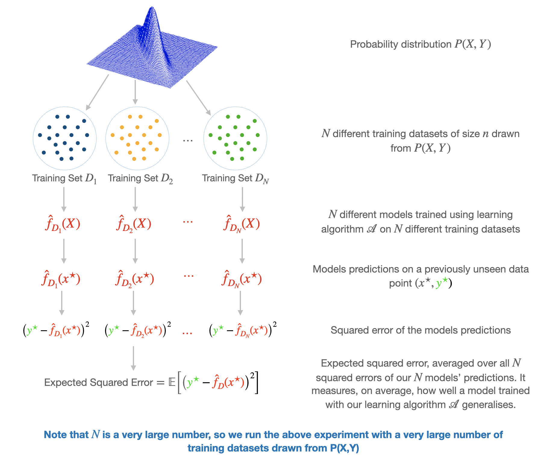
Now, because we draw our training set from a data generating distribution, it is possible, in principle³, to randomly draw a large number $N$ of different training datasets $\big(\mathcal{D}_1, \cdots, \mathcal{D}_N\big)$ of $n$ examples from the distribution. If we use the learning algorithm $\mathcal{A}$ to train a model on each training set, we will get $N$ different models $\big({\color{red}\hat f_\mathcal{D_1}(X)}, \cdots, {\color{red}\hat f_\mathcal{D_N}(X)}\big)$ that will give us $N$ different predictions $\big({\color{red}\hat f_\mathcal{D_1}(x^\star)}, \cdots, {\color{red}\hat f_\mathcal{D_N}(x^\star)}\big)$ on our arbitrary new point $x^\star$. We could calculate the squared error for each of the $N$ models predictions on $x^\star$ $\Big[\big({\color{green}y^\star} - {\color{red}\hat f_\mathcal{D_1}(x^\star)}\big)^2, \cdots, \big({\color{green}y^\star - \color{red}\hat f_\mathcal{D_N}(x^\star)}\big)^2 \big]$.
To get an idea of how well, on average, the learning algorithm $\mathcal{A}$ generalises to the previously unseen data point, we compute the mean/expectation of the squared errors of the $N$ models. This is called the expected squared error.

$$\begin{aligned} \tag{11} \text{Expected Squared Error} = \mathbb{E}\Big[\Big({\color{green}y^\star} - {\color{red}\hat f_\mathcal{D}(x^\star)}\Big)^2\Big] \end{aligned}$$

It is this expected squared error of the model that we will decompose into the bias, variance, and irreducible error components.

Expectation, Bias, and Variance of model

• Expectation of model $\mathbb{E}\big[{\color{red}\hat f_\mathcal{D}(x)}\big]$
  The expectation of the model is the average of the collection of models estimated over many training datasets.
• Bias of model $\mathbb{E}\big[{\color{red}\hat f_\mathcal{D}(x)}\big] - \color{green}f(x)$
  The model bias describes how much the expectation of the model deviates from the true value of the function $\color{green}f(x)$ we are trying to estimate. Low bias signifies that our model does a good job of approximating our function, and high bias signifies otherwise. The bias measures the average accuracy of the model.
• Variance of model $\mathbb{E}\Big[\Big({\color{red}\hat f_\mathcal{D}(x)} - \mathbb{E}\big[{\color{red}\hat f_\mathcal{D}(x)}\big]\Big)^2\Big]$
  The model variance is the expectation of the squared differences between a particular model and the expectation of the collection of models estimated over many datasets. It captures how much the model fits vary across different datasets, so it measures the average consistency of the model. A learning algorithm with high variance indicates that the models vary a lot across datasets, while low variance indicates that models are quite similar across datasets.

---

Simulation 1

In practice, the true function we try to estimate is unknown, but for the sake of demonstration, we will assume that the true function is $f(x) = sin(x)$. Individual observations of $y$ will be $y = sin(x) + \epsilon$. We assume that $\mathbb{E}[\epsilon] = 0$ and $\text{Var}(\epsilon) = \sigma^2 = 1.5$. We will sample 50 data sets each with 100 individual observations, and on them we will fit three polynomial functions of varying degrees/complexities (1, 5, 20) to estimate our true function $f(x)$. Degree 1 is the least complex and degree 20 is the most complex.

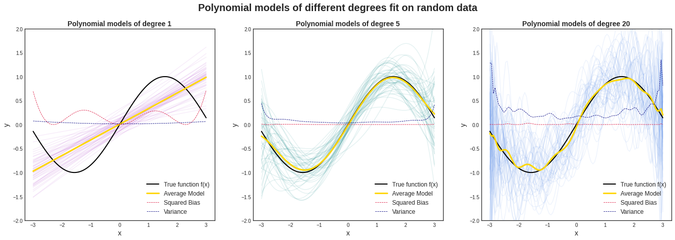
We see from the image above that on average, the degree-1 polynomial model does a bad job of estimating our true function. It has a high bias. The variance is low, which means that the model is consistent across datasets. The degree-20 polynomial model has low bias, which means it does a good job of approximating our true function, but it has a high variance. This means that the model isn’t consistent across datasets. The degree-5 polynomial model has low bias (good estimate of our true function), and a relatively low variance (consistent across datasets).

The code for this simulation can be found here.

A Note on Bias-Variance Tradeoff

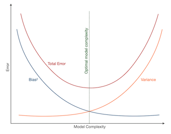
Bias-variance tradeoff is the tradeoff in attempting to simultaneously minimise the two sources of error that affect a model’s ability to generalise beyond its training set. Reducing bias generally increases variance and vice versa, and this is a function of a model’s complexity and flexibility. Low variance, high bias models tend to be less complex and less flexible and they mostly underfit the training data, while low bias, high variance models tend to be more complex with a flexible structure that tend to overfit. The optimal model will have both low bias and low variance.

---

Decomposing Expected Squared Error

As mentioned earlier, it is the expected squared error term in equation (11) that we will decompose into the bias, variance, and irreducible error components. To avoid clutter while decomposing, we will drop the $\color{green}\star$ sign from $\color{green}y^\star$ and $\color{red}(x^\star)$ from $\color{red}\hat f_\mathcal{D}(x^\star)$.

$$\tag{12} \begin{aligned} \text{Error} & = \mathbb{E}\Big[\Big({\color{green}y} - {\color{red}\hat f_\mathcal{D}}\Big)^2\Big] \\ & = \mathbb{E}\Big[\Big({\color{green}y} - {\color{red}\hat f_\mathcal{D}}\Big)\Big({\color{green}y} - {\color{red}\hat f_\mathcal{D}}\Big)\Big] \\ & = \mathbb{E}\Big[ \Big({\color{green}y}^2 - 2{\color{green}y}{\color{red}\hat f_\mathcal{D}} + {\color{red}\hat f_\mathcal{D}}^2 \Big)\Big] \\ & = \underbrace{\mathbb{E}\Big[ {\color{green}y}^2 \Big]}_{1} + \underbrace{\mathbb{E}\Big[ {\color{red}\hat f_\mathcal{D}}^2 \Big]}_{2} - \underbrace{2\mathbb{E}\Big[ {\color{green}y}\Big]\mathbb{E}\Big[ {\color{red}\hat f_\mathcal{D}} \Big]}_{3} \end{aligned}$$

Equation (12) has three terms that we will deal with separately. If we consider the third term first, we know that $\mathbb{E}\big[ {\color{red}\hat f_\mathcal{D}} \big]$ is the expectation of our model. If we recall equations (2) and (9) and that $\mathbb{E}[{\boldsymbol\epsilon}] = 0$, we can rewrite $\mathbb{E}\big[ {\color{green}y}\big]$ as:

$$\tag{13} \begin{aligned} \mathbb{E}\Big[ {\color{green}y}\Big] & = \mathbb{E}\Big[ {\color{green}f(x) + \epsilon }\Big] \\ & = \mathbb{E}\Big[ {\color{green}f(x) }\Big] + \mathbb{E}\Big[ {\color{green} \epsilon }\Big] \\ & = {\color{green}f(x)} \end{aligned}$$

For the first and second terms, we use equations (7), (9), and (13) to rewrite them as:

$$\tag{14} \begin{aligned} \mathbb{E}\Big[ {\color{green}y}^2 \Big] & = \mathbb{E}\Big[\Big({\color{green}y} - {\mathbb{E}[{\color{green}y}]}\Big)^2\Big] + {\mathbb{E}[{\color{green}y}]}^2 \\ & = \mathbb{E}\Big[\Big({\color{green}f(x) + \epsilon } - {\color{green}f(x)}\Big)^2\Big] + {\color{green}f(x)}^2 \\ & = \mathbb{E}\Big[{\color{green}\epsilon}^2 \Big] + {\color{green}f(x)}^2 \\ \mathbb{E}\Big[ {\color{red}\hat f_\mathcal{D}}^2 \Big] & = \mathbb{E}\Big[\Big({\color{red}\hat f_\mathcal{D}} - {\mathbb{E}\big[{\color{red}\hat f_\mathcal{D}}\big]}\Big)^2\Big] + {\mathbb{E}\big[{\color{red}\hat f_\mathcal{D}}\big]}^2 \end{aligned}$$

Substituting equations (13) and (14) into equation (12), we get:

$$\tag{15} \begin{aligned} \text{Error} & = \mathbb{E}\Big[ {\color{green}y}^2 \Big] + \mathbb{E}\Big[ {\color{red}\hat f_\mathcal{D}}^2 \Big] - 2\mathbb{E}\Big[ {\color{green}y}\Big]\mathbb{E}\Big[ {\color{red}\hat f_\mathcal{D}} \Big] \\ & = \mathbb{E}\Big[{\color{green}\epsilon}^2 \Big] + {\color{green}f(x)}^2 + \mathbb{E}\Big[\Big({\color{red}\hat f_\mathcal{D}} - {\mathbb{E}\big[{\color{red}\hat f_\mathcal{D}}\big]}\Big)^2\Big] + {\mathbb{E}\big[{\color{red}\hat f_\mathcal{D}}\big]}^2 - 2{\color{green}f(x)}\mathbb{E}\big[ {\color{red}\hat f_\mathcal{D}} \big] \end{aligned}$$

If we rearrange equation (15) and use expansion of squares $(a-b)^2 = a^2 - 2ab + b^2$, we get:

$$\tag{16} \begin{aligned} \text{Error} & = \underbrace{ {\mathbb{E}\big[}{\color{red}\hat f_\mathcal{D}} {\big]} ^2 - 2{\color{green}f(x)}\mathbb{E}\big[{\color{red} \hat f_\mathcal{D}}\big] + {\color{green}f(x)}^2 }_{1} + \underbrace{\mathbb{E}\Big[\Big({\color{red}\hat f_\mathcal{D}} - {\mathbb{E}[{\color{red}\hat f_\mathcal{D}}]}\Big)^2\Big]}_{2} + \underbrace{\mathbb{E}\Big[{\color{green}\epsilon}^2 \Big]}_{3} \\ & = \underbrace{\Big( {\mathbb{E}\big[}{\color{red}\hat f_\mathcal{D}} \big] - {\color{green}f(x)} \Big)^2}_{1} + \underbrace{\mathbb{E}\Big[\Big({\color{red}\hat f_\mathcal{D}} - {\mathbb{E}[{\color{red}\hat f_\mathcal{D}}]}\Big)^2\Big]}_{2} + \underbrace{\mathbb{E}\Big[{\color{green}\epsilon}^2 \Big]}_{3} \\ & = \underbrace{\Big( {\mathbb{E}\big[}{\color{red}\hat f_\mathcal{D}} \big] - {\color{green}f(x)} \Big)^2}_{\text{Bias}^2 \space \text{of model}} + \underbrace{\mathbb{E}\Big[\Big({\color{red}\hat f_\mathcal{D}} - {\mathbb{E}[{\color{red}\hat f_\mathcal{D}}]}\Big)^2\Big]}_{\text{Variance of model}} + \underbrace{\sigma^2}_{\text{Irreducible error}} \end{aligned}$$

And there is the error decomposed into its three constituent parts. To see a breakdown of how the third term $\mathbb{E}\Big[{\color{green}\epsilon}^2 \Big]$ became $\sigma^2$, you can check the footnote.⁴

Illustrating Bias-Variance Decomposition using simulated data

In Simulation 1, we estimated our true function $f(x) = sin(x)$ by fitting three polynomial functions of varying complexities. What we really care about though is how our models perform on previously unseen data. In this section, we will demonstrate this and show how the expected squared error decomposes into the sum of variance and squared bias by running the following steps:

• Generate 100 random datasets of 500 observations each from $sin(x) + \epsilon$. We assume that the $\text{Var}(\epsilon) = \sigma^2 = 1.5$.
• Split the generated datasets into training and test sets.
• Fit 20 polynomial functions (degrees from 1 to 20) on each of the training sets.
• Predict the value of the test set using the fitted models.
• Calculate the expected prediction error (the mean squared error) on the test set for each model.
• Show the expected prediction error as a sum of the variance and squared bias.

---

Simulation 2

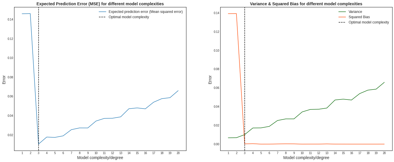
We see from graph on the left in the image above that the error starts quite high, drops off to its minimum at model complexity 3, and then starts climbing rapidly as the complexity increases. If we look at the right graph, we see that it follows the bias-variance tradeoff. The squared-bias of the models drops as the complexity increases, but variance increases. Low bias, high variance models suggest that the models overfit the training data and hence performs poorly on the test data. Our optimal model has low bias and low variance and it is the model with complexity 3 in our simulation.

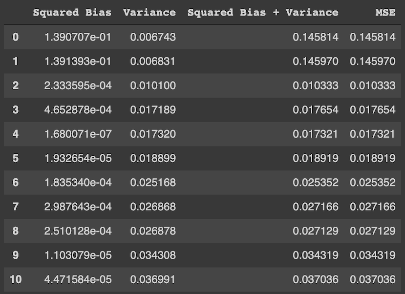
We see from the table above that the mean squared error (MSE) is a sum of the squared bias and the variance, as shown in equation (16). The irreducible part of the decomposition is not added to our sum because we cannot estimate it from data.

The code for this simulation can be found here.

---

Conclusion

We have shown the decomposition of the generalisation error for regression problems. It is possible to show this decomposition for classification problems. Pedro Domingos’ brilliant paper, A Unified Bias-Variance Decomposition and its Application goes over it in details.

Footnotes

Footnotes

1. Expected value explained on Brilliant.org ↩

2. Independent and Identically Distributed Random Variables ↩

3. In practice, we have access to only one training dataset. ↩

4. Using the variance lemma in equation (7) and the assumption that $\mathbb{E}[\boldsymbol \epsilon] = 0$ and $\text{Var}(\boldsymbol \epsilon) = \sigma^2$: $\begin{aligned} \mathbb{E}\big[{\boldsymbol \epsilon}^2 \big] & = \text{Var}(\boldsymbol \epsilon) + \mathbb{E}[\boldsymbol \epsilon]^2 = \sigma^2 \end{aligned}$. ↩