Deriving Machine Learning Cost Functions using Maximum Likelihood Estimation (MLE) - Part II

In Part I of this article, we introduced Maximum Likelihood Estimation (MLE), Likelihood function, and derived Mean Squared Error (MSE) using Maximum likelihood estimation. In this article, we will use Maximum likelihood estimation to derive Cross-Entropy cost function, which is commonly used for binary classification problems.

Background

Binary logistic regression is used to model the relationship between a categorical target variable $Y$ and a predictor vector $X = (X_1, X_2, \cdots, X_p)$. The target variable will have two possible values, such as whether a student passes an exam or not, or whether a visitor to a website subscribes to the website’s newsletter or not. The two possible categories are coded as ‘1’, called the positive class, and ‘0’, called the negative class. Binary logistic regression estimates the probability that the response variable $Y$ belongs to the positive class given $X$.

$$\tag{1} \begin{aligned} p(X) = Pr(Y = 1 | X) \end{aligned}$$

In linear regression, we model the expected value (the mean $\mu$) of the continuous target variable $Y$ as a linear combination of the predictor vector $X$ and estimate the weight parameters $\beta_1, \beta_2, \cdots, \beta_p$ using our training data.

$$\tag{2} \begin{aligned} \mathbb{E}(Y|X) = \beta_0 + \beta_1 X_1 + \cdots + \beta_p X_p \end{aligned}$$

In this case where our target variable $Y$ is categorical and has two possible values coded as 0 and 1, the expected value or mean of $Y$ is the probability $p(X)$ of observing the positive class¹. It seems sensible then to model the expected value of our categorical $Y$ variable using equation (2), as in linear regression.

$$\tag{3} \begin{aligned} \mathbb{E}(Y|X) = p(X) = \beta_0 + \beta_1 X_1 + \cdots + \beta_p X_p \end{aligned}$$

The problem with modelling the probability $p(X)$ as a linear combination of the predictor variables is that probability $p(X)$ has a range $[0, 1]$, but the right-hand side of the equation outputs values in the range $(-\infty, +\infty)$. In other words, we will get meaningless estimates of the probability if we use that equation.
The solution is to use a function of probability $p(X)$ that provides a suitable relationship between the linear combination of the predictor variables $X$ and $p(X)$, the mean of the response variable. This function is called a link function, and it maps the probability range $[0, 1]$ to $(-\infty, +\infty)$.
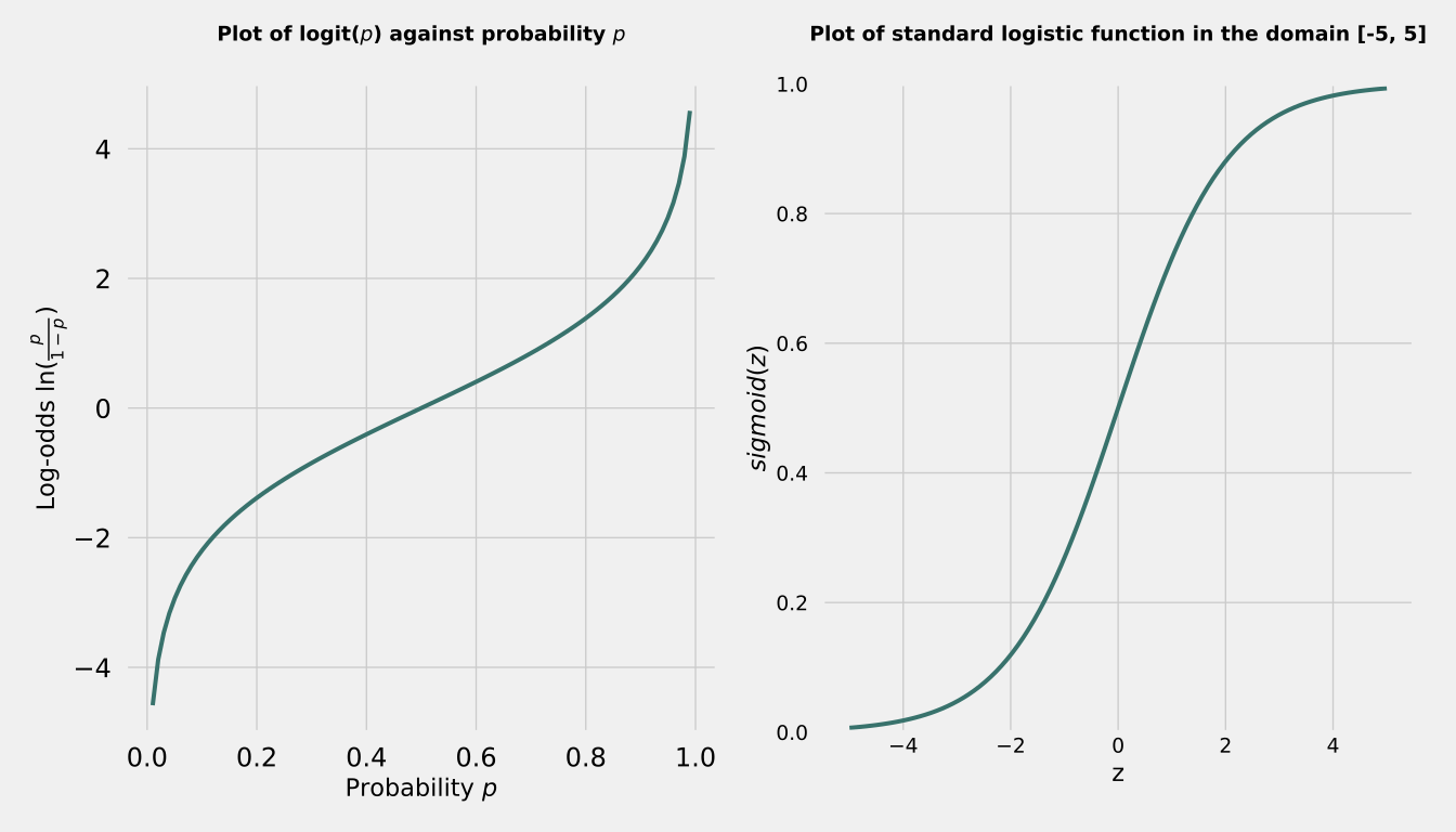
The most commonly used link function for binary logistic regression is the logit function (or log-odds²), given as:

$$\tag{4} \begin{aligned} \text{logit}\bigg(p(X)\bigg) = \text{log}\bigg(\frac{p(X)}{1-p(X)}\bigg) = \beta_0 + \beta_1 X_1 + \cdots + \beta_p X_p \end{aligned}$$

How do we then go from the logit function to getting the estimate of the probability p(X) of observing the positive class? Because logit is a function of probability, we can take its inverse to map arbitrary values in the range $(-\infty, +\infty)$ back to the probability range $[0, 1]$.
Recall that the inverse function of the natural logarithm function is the exponential function, so if we take the inverse of equation (4), we get:

$$\tag{5} \begin{aligned} \frac{p(X)}{1-p(X)} = e^{(\beta_0 + \beta_1 X_1 + \cdots + \beta_p X_p)} \end{aligned}$$

If we solve for $p(X)$ in equation (5), we get³:

$$\tag{6} \begin{aligned} p(X) & = \frac{e^{(\beta_0 + \beta_1 X_1 + \cdots + \beta_p X_p)}}{e^{(\beta_0 + \beta_1 X_1 + \cdots + \beta_p X_p)} + 1} \\ & = \frac{1}{1 + e^{(-\beta_0 + \beta_1 X_1 + \cdots + \beta_p X_p)}} \end{aligned}$$

Equation (6) is the logistic (or sigmoid) function, and it maps values in the logit range $(-\infty, +\infty)$ back into the range $[0, 1]$ of probabilities.

Deriving Cost Entropy using MLE

Given a set of $n$ training examples $\\{(x^{(1)}, y^{(1)}), (x^{(2)}, y^{(2)}), \cdots, (x^{(n)}, y^{(n)})\\}$, binary cross-entropy is given by:

$$\tag{7} \begin{aligned} \text{Cross-Entropy} = -\bigg[\frac{1}{n} \sum_{i=1}^n\bigg(y^{(i)}\text{log} p^{(i)} + (1- y^{(i)})\text{log}(1 - p^{(i)})\bigg)\bigg] \end{aligned}$$

where $x^{(i)}$ is the feature vector, $y^{(i)}$ is the true label (0 or 1) for the $i^{th}$ training example, and $p^{(i)}$ is the predicted probability that the $i^{th}$ training example belongs to the positive class, that is, $Pr(Y = 1 | X = x^{(i)})$.

In this section, we will derive cross-entropy using MLE. If you are not already familiar with MLE and likelihood function, I will advise that you read the section that explains both concepts in Part I of this article.

The derivation of cross-entropy follows from using MLE to estimate the parameters $\beta_0, \beta_1, \cdots, \beta_p$ of our logistic model on our training data.
We start by describing the random process that generated $y^{(i)}$.
$y^{(i)}$ is a realisation of the Bernoulli random variable⁴ $Y$. The Bernoulli distribution is parameterised by $p$, and its probability mass function (pmf) is given by:

$$\tag{8} \begin{aligned} Pr(Y = y^{(i)}) = \begin{cases} p & \text{if } y^{(i)} = 1, \\ 1-p & \text {if } y^{(i)} = 0. \end{cases} \end{aligned}$$

which can be written in the more compact form:

$$\tag{9} \begin{aligned} Pr(Y = y^{(i)}) = p^{y^{(i)}}(1-p)^{1 - y^{(i)}} \ \text{for} \ y^{(i)} \in \{0,1\} \end{aligned}$$

We then define our Likelihood function. The estimates of $\beta_0, \beta_1, \cdots, \beta_p$ we choose will be the ones that maximise the likelihood function. The likelihood function is a function of our parameter $p$ given our training data:

$$\tag{10} \begin{aligned} \mathcal{L}(p | (x^{(1)}, y^{(1)}), (x^{(2)}, y^{(2)}), \cdots, (x^{(n)}, y^{(n)})) & = \prod_{i=1}^n f(y^{(i)}|p) \\ & = \prod_{i=1}^n p^{y^{(i)}}(1-p)^{1 - y^{(i)}} \end{aligned}$$

It is easier to work with the log of the likelihood function⁵, called the log-likelihood, so if we take the natural logarithm of equation (10), we get:

$$\tag{11} \begin{aligned} \log \bigg(\mathcal{L}(p | y^{(1)}, y^{(2)}, \cdots, y^{(n)})\bigg) & = \log\bigg( \prod_{i=1}^n p^{y^{(i)}}(1-p)^{1 - y^{(i)}} \bigg) \\ & = \sum_{i=1}^n \log \bigg(p^{y^{(i)}}(1-p)^{1 - y^{(i)}}\bigg) \\ & = \sum_{i=1}^n \bigg(y^{(i)}\text{log}p^{(i)} + (1-y^{(i)})\text{log}(1-p^{(i)})\bigg) \end{aligned}$$

Recall that for our training data, $p^{(i)}$ in equation (11) is the predicted probability of the $i^{th}$ training example gotten from the logisitic function, so it is a function of the parameters $\beta_0, \beta_1, \cdots, \beta_p$. The maximum likelihood estimate $\hat \beta$ is therefore the value of the parameters that maximises the log-likelihood function.

$$\tag{12} \begin{aligned} \hat \beta = \underset{\beta}{\operatorname{arg\,max}} \bigg[ \sum_{i=1}^n \bigg(y^{(i)}\text{log}p^{(i)} + (1-y^{(i)})\text{log}(1-p^{(i)})\bigg) \bigg] \end{aligned}$$

We also know that maximising a function is the same as minimising its negative.

$$\tag{13} \begin{aligned} \hat \beta = \underset{\beta}{\operatorname{arg\,min}} \bigg[ -\sum_{i=1}^n \bigg(y^{(i)}\text{log}p^{(i)} + (1-y^{(i)})\text{log}(1-p^{(i)})\bigg) \bigg] \end{aligned}$$

Taking the average across our $n$ training examples, we get:

$$\tag{14} \begin{aligned} \hat \beta = \underset{\beta}{\operatorname{arg\,min}} \bigg[\color{red}-\frac{1}{n}\sum_{i=1}^n \bigg(y^{(i)}\text{log}p^{(i)} + (1-y^{(i)})\text{log}(1-p^{(i)})\bigg) \color{black}\bigg] \end{aligned}$$

which is the cross-entropy as defined in equation (7).

Footnotes

Footnotes

1. $Y$ is a Bernoulli random variable. The Bernoulli distribution is a discrete probability distribution that describes processes that have only two possible outcomes: 1, with a probability of $p$ and 0, with a probability of $1 - p$. The expectation (or mean) of the Bernoulli distribution is $p$. [Proof] ↩

2. The odds is defined as the ratio of the probability $p$ of observing an event to the probability $1-p$ of not observing that event. $\text{odds} = \frac{p}{1-p}$. If, for example, the odds of an event happening is $o$:1, it means that the event happened $o$ times out of a total of $o+1$ occurrences. The log-odds is simply the natural logarithm of the odds. ↩

3. A simple derivation can be found here ↩

4. Bernoulli distribution is the discrete probability distribution of a random variable that takes on two possible values: 1 with probability $p$ and 0 with probability $1-p$. An experiment modelled by the Bernoulli distribution is called a Bernoull trial. Examples of Bernoulli trials include: tossing a coin (head/tail), playing a game (winning/not winning). ↩

5. The reasons why this is the case is explained clearly in Part I. Check the ‘What is Maximum Likelihood Estimation?’ section. ↩